Adsorber Design : Some Basic Principles
Introduction:
When a gas or a liquid comes in contact with a solid, the molecules are concentrated in the interface due to their interaction with the solid surface. This increase in concentration of molecules on the solid surface is called adsorption. Since the adsorbed molecules are often held very weakly by the solid, the adsorbent bed is regenerated easily by heating, or by reduction of pressure, and / or by a flow of a purge fluid. In case the adsorption is strong, the regeneration requires chemical treatment. This preferential concentration of an adsorbate on the solid surface and the regeneration of the adsorbent is the basis of the adsorption technology, which is now used very effectively in the separation and purification of many gaseous and liquid mixtures.
A majority of the industrial applications of adsorption use fixed bed adsorbers. With a single adsorber, the process is batch type only. For continuous operation the simplest configuration must have at least two adsorbers operating in tandem where one adsorber is on adsorption mode and the other is on regeneration. In certain applications, the bed instead of being fixed, may move with respect to the feed or the input and output flows are controlled in such manner that a movement of the bed is simulated with respect to the feed. This is called simulated moving bed (SMB), and is practiced in many critical liquid phase separations.
The fixed bed adsorption processes are classified and designed on the basis of the technology used for regeneration. When the regeneration is done by a change in pressure, the process is Pressure Swing Adsorption or simply PSA. Often the depressurization is followed by evacuation for better recovery, and such processes are called Vacuum Swing Adsorption (VSA) or Vacuum Pressure Swing Adsorption (VPSA) depending upon the combination of vacuum and pressure. In case the regeneration is by heating, the process is called Thermal Swing Adsorption or TSA. The choice of a particular regeneration process and the adsorbent depends upon the various engineering aspects of the process and its economics.1
The design of an adsorber is quite complex, and beyond the scope of such a brief article. Basically, it involves the balancing of heat and mass at every elemental section of the adsorber, and the solution of the resultant partial differential equation. The problem is complicated by the fact that the adsorption being an exothermic process, the elemental section cannot be treated strictly as isothermal. Similarly further simplification is not possible, if the axial dispersion is not negligible. However, many analytical solutions are available in the literature for specific adsorption models2 and some approximate solutions also are practiced on the basis of certain assumptions. On many occasions these approximate treatments yield a reasonably accurate design in much less time3. This article deals with some of these less rigorous, procedures, used for designing Thermal Swing type adsorber units. The design principles of PSA units are different4, and are not dealt in this article.
The basic design equation:
Consider an elemental section of an
adsorber (Fig.1). A feed enters the bed with the contaminant (adsorbate)
concentration, ![]() , and as it passes through the
elemental section of length
, and as it passes through the
elemental section of length ![]() , the concentration of the
contaminant decreases by
, the concentration of the
contaminant decreases by ![]() , while the quantity of the adsorbed
phase on the adsorbent increases by
, while the quantity of the adsorbed
phase on the adsorbent increases by ![]() .
.

Fig. 1 An Elemental Section of an Adsorber
The mass balance equation within this elemental section may be written as:
![]() ……. (1)
……. (1)
where ![]() = axial dispersion coefficient, m2/s,
= axial dispersion coefficient, m2/s, ![]() = bed voidage or porosity of the adsorbent bed,
= bed voidage or porosity of the adsorbent bed, ![]() = quantity (mol) adsorbed per unit
mass of the adsorbent,
= quantity (mol) adsorbed per unit
mass of the adsorbent,![]() interstitial velocity =
interstitial velocity = ![]() m/s,
m/s, ![]() = the rate of feed flow, m3/s,
ρS = true density of the adsorbent, kg/dm3 and
= the rate of feed flow, m3/s,
ρS = true density of the adsorbent, kg/dm3 and ![]() = the cross-section of the bed, m2.
= the cross-section of the bed, m2.
Since most adsorption processes are
quite fast and only limited by mass transfer, there is no concentration
gradient within the particles, and the quantity of the adsorbed phase ![]() becomes equal to the quantity of
adsorbed phase in equilibrium with the feed
becomes equal to the quantity of
adsorbed phase in equilibrium with the feed ![]() , if the adsorbent particles are
sufficiently small with a large diffusion coefficient. In that case the right
hand side of equation (1), viz. the term for axial dispersion, becomes zero,
and the equation (1) reduces to:
, if the adsorbent particles are
sufficiently small with a large diffusion coefficient. In that case the right
hand side of equation (1), viz. the term for axial dispersion, becomes zero,
and the equation (1) reduces to:
![]() ……… (2)
……… (2)
This equation (2), after a little mathematical manipulation, gives the ideal breakthrough time as:
 =
=  ……… (3)
where, ![]() bulk density of the adsorbent, kg/dm3.
The term
bulk density of the adsorbent, kg/dm3.
The term ![]() in equation (3) may be derived from
the adsorption isotherm and provides a simple basis for estimating the
breakthrough time, and hence the bed volume. The procedure has been illustrated
by Coulson et al5 for different adsorption isotherms.
in equation (3) may be derived from
the adsorption isotherm and provides a simple basis for estimating the
breakthrough time, and hence the bed volume. The procedure has been illustrated
by Coulson et al5 for different adsorption isotherms.
Design of adsorber on the basis of Transfer Units:
Another simple procedure is followed in
the design of a moving bed adsorber. Let us consider Fig.1 again. The mass removed from the feed
within the elemental section dZ = ![]() , and the mass build-up an the adsorbent surface =
, and the mass build-up an the adsorbent surface = ![]() , where
, where ![]() rate constant for adsorption of
component A, m s-1,
rate constant for adsorption of
component A, m s-1, ![]() external surface area of the particle
per unit volume of the adsorbent bed, m-1, and
external surface area of the particle
per unit volume of the adsorbent bed, m-1, and ![]() = concentration of the component A on
the solid surface, kmol/m3. Thus, the mass balance may be written
as:
= concentration of the component A on
the solid surface, kmol/m3. Thus, the mass balance may be written
as:
![]() =
= ![]() …… (4)
…… (4)
Since the rate of adsorption is very
fast, the concentration of the adsorbed molecules A on the solid surface, ![]() =
= ![]() , where
, where ![]() is the adsorbate concentration in equilibrium with the mean
adsorbed phase concentration. So the total length of the bed may be obtained by
integration of dZ,
is the adsorbate concentration in equilibrium with the mean
adsorbed phase concentration. So the total length of the bed may be obtained by
integration of dZ,
![]() ……. (5)
……. (5)
which may be expressed as ![]() where
where ![]() = number of transfer units =
= number of transfer units = ![]() and
and ![]() = height of a transfer unit =
= height of a transfer unit = ![]() .
.
The calculation procedure consists of (a) drawing an operating line on the basis of the inlet and outlet concentrations of the contaminant in the feed and the initial and final loading of the contaminant on the adsorbent as the adsorbent comes in contact with the feed and as it leaves the feed, respectively, (b) drawing an adsorption isotherm, and then (c) calculation of the height of the transfer units (similar to the calculation of HETP in distillation). The procedure has been illustrated by Pavlov et al.6
Adsorption capacity:
The adsorption capacity of an
adsorbent for a particular adsorbate are estimated in two ways: equilibrium
adsorption capacity, and dynamic adsorption capacity, and both data
are important in the design. The equilibrium adsorption capacity is
measured by keeping the adsorbent in contact with the adsorbate until
equilibrium is reached, and is represented by plots of ![]() vs equilibrium partial pressure
vs equilibrium partial pressure![]() or
or ![]() vs. the residual concentration
vs. the residual concentration![]() of the adsorbate in equilibrium with
the adsorbent (adsorption isotherms). Instead of measuring the
isotherm, which is a time consuming and expensive exercise, the equilibrium
adsorption data may be taken from the published database7, where
possible. In case of the non-availability of such data, the isotherm may be
constructed by a very simple procedure6 on the basis of the known
isotherm of a standard substance, provided both substances are of similar
chemical nature. Presently, the equilibrium measurements are available for
mostly single components because a satisfactory analytical model does not exist
for mixtures.
of the adsorbate in equilibrium with
the adsorbent (adsorption isotherms). Instead of measuring the
isotherm, which is a time consuming and expensive exercise, the equilibrium
adsorption data may be taken from the published database7, where
possible. In case of the non-availability of such data, the isotherm may be
constructed by a very simple procedure6 on the basis of the known
isotherm of a standard substance, provided both substances are of similar
chemical nature. Presently, the equilibrium measurements are available for
mostly single components because a satisfactory analytical model does not exist
for mixtures.
As it has been shown in equation (3), the analytical form of the isotherm is important in the calculation of breakthrough time, and hence of adsorbent capacity. At present four different models, namely, (a) Langmuir, (b) Freundlich, (c) Brunauer, Emmett and Teller (BET), and (d) Dubinin-Radushkevich (DR) are commonly used in the analysis of isotherms, but twelve other models are also in vogue8.
The dynamic adsorption capacity is measured in the laboratory by passing the feed mixture over a small bed of adsorbent, designed by simulating the actual application conditions, until the breakthrough occurs. It is given by:
 …………… (6)
where ![]() = dynamic adsorption capacity, kg/kg
of the adsorbent,
= dynamic adsorption capacity, kg/kg
of the adsorbent, ![]() = relative molar mass of the
adsorbate, kg/kmol,
= relative molar mass of the
adsorbate, kg/kmol, ![]() = volume of the adsorbent bed, m3,
= volume of the adsorbent bed, m3,
![]() bulk density of the adsorbent, kg/dm3
, and
bulk density of the adsorbent, kg/dm3
, and ![]() = time at which the bed is
stoichiometrically saturated, s. (See Fig.2, which is further explained in the
next section.)
= time at which the bed is
stoichiometrically saturated, s. (See Fig.2, which is further explained in the
next section.)

Fig. 2 Breakthrough Curve with time9
The dynamic adsorption capacity is a very important quantity and gives a good idea about the adsorbent’s performance. It is always less than the equilibrium adsorption capacity, and called also as effective adsorption capacity. For liquid phase adsorption on microporous adsorbents like activated carbon with a long residence time, the effective adsorption capacity may be 80-90% of the equilibrium adsorption capacity, but for many gas phase adsorptions, it may be 10-20% only. Sometimes in absence of other reliable data, an adsorber is designed by simple scale up computation on the basis of this dynamic adsorption capacity with a reasonable margin.
When should a bed be regenerated?
Let us consider now a fixed bed of
adsorbent through which the feed containing the adsorbate is passed at a rate
of ![]() , m3/s. As the feed comes
in contact with an elemental section of the adsorbent (Fig.1), it becomes
saturated with the adsorbate at that instant, since the adsorption is considered
as a fast process. Therefore, the residual adsorbate, if any, flows to the next
section. As more adsorbate flows, the next section becomes saturated. Thus
there happens to be a concentration profile of adsorbate as adsorbed on the
adsorbent and this profile moves along the length of the adsorbent bed. This is
shown schematically in Fig. 3.
, m3/s. As the feed comes
in contact with an elemental section of the adsorbent (Fig.1), it becomes
saturated with the adsorbate at that instant, since the adsorption is considered
as a fast process. Therefore, the residual adsorbate, if any, flows to the next
section. As more adsorbate flows, the next section becomes saturated. Thus
there happens to be a concentration profile of adsorbate as adsorbed on the
adsorbent and this profile moves along the length of the adsorbent bed. This is
shown schematically in Fig. 3.

Fig.3 The progress of concentration profile through the adsorbent bed9
The section of the bed through which
the concentration of the adsorbate changes from ![]() to
to ![]() is known as Mass Transfer Zone or
simply as MTZ (Fig. 2).
is known as Mass Transfer Zone or
simply as MTZ (Fig. 2). ![]() is the concentration of the
contaminant (adsorbate) in the feed, and
is the concentration of the
contaminant (adsorbate) in the feed, and ![]() is the desired (design or final)
concentration of the contaminant in the outlet as the feed exits from the
adsorber. The progress of adsorption is thus the same as the progress of the
MTZ along the bed. As the MTZ touches the end of the bed (stage 6 in Fig.3),
breakthrough occurs. That means, the exit concentration of the adsorbate starts
increasing from
is the desired (design or final)
concentration of the contaminant in the outlet as the feed exits from the
adsorber. The progress of adsorption is thus the same as the progress of the
MTZ along the bed. As the MTZ touches the end of the bed (stage 6 in Fig.3),
breakthrough occurs. That means, the exit concentration of the adsorbate starts
increasing from ![]() , and very soon it becomes equal to
the inlet concentration,
, and very soon it becomes equal to
the inlet concentration, ![]() , indicating that no further
adsorption takes place. This is shown in Figs.3 & 4. However, the bed
should not be kept in operation till this point (
, indicating that no further
adsorption takes place. This is shown in Figs.3 & 4. However, the bed
should not be kept in operation till this point (![]() of Fig. 3) is reached, as the
concentration of the adsorbate exceeds the design limit at time
of Fig. 3) is reached, as the
concentration of the adsorbate exceeds the design limit at time ![]() (Fig. 3), called as breakthrough
time or breakpoint time, when the bed should be switched to
regeneration.
(Fig. 3), called as breakthrough
time or breakpoint time, when the bed should be switched to
regeneration.
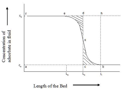
Fig.4 Breakthrough Curve along the Length of the Bed9
The MTZL (length of MTZ) is one of the most important parameter characterizing the performance of the bed. In case the MTZ is very narrow and moves very slowly, the adsorbent bed would have a very long cycle time. That means it may be operated without regeneration for a long time. On the contrary, if the MTZ is very broad and moves very fast, then the particular bed would have a very short cycle and may not be economical to operate at all. Often it is therefore a major exercise in adsorber design to calculate the MTZ and its propagation time.
A simple procedure for the estimation of MTZ is now described below. The used adsorbent capacity is represented by the area fesbaf (Fig. 4), which is equal to the area of the rectangle, fdca, since the stoichiometric point s is at the mid-point of the breakthrough line, esb. This is equal to the length of the equivalent equilibrium bed, LES. The unused adsorbent bed capacity is represented therefore by the area esbhe, which is equal to the area of the rectangle, cdhb. This is equal to the length of the unutilised bed or LUB. From Fig.4 with a little geometry, it may be calculated that:
 …………… (7)
The LUB is thus a fraction of the total bed length, and may be determined in the laboratory with any bed length by a single experiment from the breakthrough curve. This approach is applicable only for systems showing favourable isotherms, particularly Type I, and the configuration of the laboratory scale equipment should be similar to that of the full scale unit10. According to some thumb rules, the LUB is a fixed proportion of the MTZL.
The size and shape of the MTZ are crucial. In case the rate of mass transfer is very fast and equal to or higher than the rate of adsorption, the shape of the concentration profile is that of a “shock wave” (MTZ1 of Fig.5), as the rate of mass transfer becomes less, the length of the MTZ increases (MTZ2 and MTZ3 of Fig.5), consequently increasing the length of the adsorbent bed itself. The estimation of MTZL (length of mass transfer zone) by actual experiment in the laboratory or pilot plant after simulating the actual plant conditions or by calculation on the basis of kinetic and mass transfer data is therefore a major exercise in the design of adsorber. The MTZL is estimated from the breakthrough curve (Fig.3).
 …. ….. (9)
Pavlov et al7 have given
some excellent examples of calculating the MTZL, and breakpoint time ![]() for the adsorption of organic
substances on activated carbons. Thomas and Crittendon10 also have
discussed various methods of measuring MTZL, which are used in water industry
for the adsorption of organic
substances on activated carbons. Thomas and Crittendon10 also have
discussed various methods of measuring MTZL, which are used in water industry

Fig.5 The changing shape of Mass Transfer Zone (MTZ) with rate of mass transfer
Single Bed or Multi Bed?
In many organic chemical or pharmaceutical industries there is a need to recover one or more components from a mixture of liquids or to dry a solvent, which has been contaminated with water. Often such separations are carried out in batches using activated alumina, activated carbon or molecular sieve as adsorbent. In case of batch operation, the adsorbent is added in the form of powder, beads, pellets or granules to the liquid containing the adsorbate(s), and the mixture is kept in contact with the adsorbent for some time, preferably with mild agitation, until the adsorption equilibrium is reached. Thereafter the adsorbent is separated from the liquid by filtration, and regenerated by suitable treatment for further use again.
Although the batch operations are
simple in principle, and can be carried out at ease in most cases, there is one
important aspect regarding the optimization of the adsorbent quantity. If the
adsorption is carried out in more than one stages, then the total quantity of
adsorbent required for all the stages is always less than the quantity
required, if the adsorption were carried out in a single stage. Further, more
the stages, the less is the total quantity, which is given by the equation (10)
for adsorptions, which obey the Henry’s law, viz. ![]() . For such cases,
. For such cases,
 …….. (10)
where ![]() = the optmised quantity of adsorbent
in the ith stage,
= the optmised quantity of adsorbent
in the ith stage, ![]() number of stages,
number of stages, ![]() = volume of the feed. In case, the
isotherm is linear, i.e. obeys Henry’s law, the quantity of adsorbent at each
stage may be equal; and given by:
= volume of the feed. In case, the
isotherm is linear, i.e. obeys Henry’s law, the quantity of adsorbent at each
stage may be equal; and given by:  …………… (11)
whereas if the isotherm is non-linear, the quantities would be different, but usually the first stage would require the largest quantity followed by less quantities in succeeding stages. The quantities required for each stage may be determined graphically from the adsorption isotherm as illustrated below (Fig. 6)
OABC is the adsorption isotherm, viz.
the plot of equilibrium adsorption, kg adsorbed / kg of adsorbent against the
equilibrium concentrations Ce in kmol/m3. Let us
assume that we want to bring down the equilibrium residual concentrations in
the solution from C0 to C1 in stage 1, from C1 to
C2 in stage 2, and from C2 to C3 in stage 3 so on. Draw a vertical line from C1 in the concentration axis to the
isotherm so that it intersects the isotherm at point C. The slope of the line C3C = ![]() , where V = volume of the
liquid mixture in m3, M = molecular weight of the adsorbate
(adsorbate), and Q1 = kg of adsorbent required for the first
stage. Similarly, draw a vertical line from C2, which intersects the
isotherm at B, and the slope of the line C1B =
, where V = volume of the
liquid mixture in m3, M = molecular weight of the adsorbate
(adsorbate), and Q1 = kg of adsorbent required for the first
stage. Similarly, draw a vertical line from C2, which intersects the
isotherm at B, and the slope of the line C1B = ![]() , and so on.
, and so on.

Fig. 6 Graphical Procedure for Estimation of Adsorbent Quantity
References:
01. N. C. Datta, “Adsorption Technology : Theory & Practice”, Chemical Industry Digest, September 2006, Vol XIX, pp.48-54
02. (a) D. M. Ruthven, Principles of Adsorption and Adsorption Processes, Wiley Interscience, New York , 1984; (b) R. T. Yang, “ Gas Separation by Adsorption Processes”, Butterworths, Boston, 1987; (c) C. Tien, “Adsorption Calculations and Modeling”, Butterworths – Heinemann, Boston, 1994.
03. (a) “Handbook of Separation Process Technology”, Edited by R. W. Rousseau, Wiley – Interscience, New York, 1987; (b) K. S. Knaebel, “A ‘How To’ Guide for Adsorber Design”, http://www.adsorption.com/publications/AdsorberDes2.pdf.
04. D. M. Ruthven, D. Farroq and K. S. Knaebel, Pressure Swing Adsorption, VCH Wiley, New York, 1994..
05. J. M. Coulson, J. F. Richardson, J. R. Backhurst, and J. H. Harker, Chemical Engineering: Particle Technology and Separation Processes, Butterworth-Heinemann, London, 1991, Vol 2, Chapter 17.
06. K. F. Pavlov, P. G. Romankov, and A. A. Noskov, “Example and Problems to the Course of Unit Operations of Chemical Engineering”, (Translated from the Russian by G. Leib), Mir Publishers, Moscow, 1979, Chapter 9.
07. (a) D. P. Valenzuela and A. L. Myers, “Adsorption Equilibrium Data Book”, Prentice Hall, Engelwood Cliffs, 1989; (b) R. A. Dobbs and J. M. Cohen, “Carbon Isotherms for Toxic Organics”, Document No. EPA-600/8-80-023, U.S. Environment Protection Agency, 1980 (May be obtained or downloaded from the web site of National Service Center for Environmental Publications (NCSEP) (http://nepis.epa.gov)
08. K. S. Knaebel, “Adsorbent Selection”, Table 2, p. 14, Source:
http://www.adsorption.com/publications/AdsorbentSel1B.pdf,
09. W. J. Thomas, and B. D. Crittendon, “Adsorption Technology and Design”, Butterworth- Heinemann, London, 1998, Chapter 5.
10. W. J. Thomas, and B. D. Crittendon, ibid., p.165.
11. J. S. Mattson, and H. B. Mark, “Activated Carbon: Surface Chemistry and Adsorption from Solution”, Marcel Dekker, New York, 1971; “Carbon Adsorption Handbook”, Edited by P. N. Cheremisinoff and F. Ellerbusch, Ann Arbor Science, Ann Arbor, 1978.
12. “Treatment of Water by Granular Activated Carbon”, Edited by M. J. McGuire and I. H. Suffet, American Chemical Society, Advances in Chemistry Series No. 202, Washington, 1983.; S. D. Faust and O. M. Aly, “Adsorption Processes for Water Treatment”, Butterworths, Boston, 1987.